如何通过Python来开始数据分析

最近，Analysis with Programming加入了Planet Python。作为该网站的首批特约博客，我这里来分享一下如何通过Python来开始数据分析。具体内容如下：

数据导入——导入本地的或者web端的CSV文件; 数据变换; 数据统计描述; 假设检验——单样本t检验; 可视化; 创建自定义函数。

数据导入

这是很关键的一步，为了后续的分析我们首先需要导入数据。通常来说，数据是CSV格式，就算不是，至少也可以转换成CSV格式。在Python中，我们的操作如下：

1 2 3 4 5 6 7 8 import pandas as pd # Reading data locally df = pd.read_csv(/Users/al-ahmadgaidasaad/Documents/d.csv) # Reading data from web data_url = "https://raw.githubusercontent.com/alstat/Analysis-with-Programming/master/2014/Python/Numerical-Descriptions-of-the-Data/data.csv" df = pd.read_csv(data_url)

为了读取本地CSV文件，我们需要pandas这个数据分析库中的相应模块。其中的read_csv函数能够读取本地和web数据。

数据变换

既然在工作空间有了数据，接下来就是数据变换。统计学家和科学家们通常会在这一步移除分析中的非必要数据。我们先看看数据：

1 2 3 4 5 6 7 8 9 10 11 12 13 14 15 16 17 18 19 20 21 # Head of the data print df.head() # OUTPUT     Abra  Apayao  Benguet  Ifugao  Kalinga 0   1243    2934      148    3300    10553 1   4158    9235     4287    8063    35257 2   1787    1922     1955    1074     4544 3  17152   14501     3536   19607    31687 4   1266    2385     2530    3315     8520 # Tail of the data print df.tail() # OUTPUT      Abra  Apayao  Benguet  Ifugao  Kalinga 74   2505   20878     3519   19737    16513 75  60303   40065     7062   19422    61808 76   6311    6756     3561   15910    23349 77  13345   38902     2583   11096    68663 78   2623   18264     3745   16787    16900

对R语言程序员来说，上述操作等价于通过print(head(df))来打印数据的前6行，以及通过print(tail(df))来打印数据的后6行。当然Python中，默认打印是5行，而R则是6行。因此R的代码head(df, n = 10)，在Python中就是df.head(n = 10)，打印数据尾部也是同样道理。

在R语言中，数据列和行的名字通过colnames和rownames来分别进行提取。在Python中，我们则使用columns和index属性来提取，如下：

1 2 3 4 5 6 7 8 9 10 11 # Extracting column names print df.columns # OUTPUT Index([uAbra, uApayao, uBenguet, uIfugao, uKalinga], dtype=object) # Extracting row names or the index print df.index # OUTPUT Int64Index([0, 1, 2, 3, 4, 5, 6, 7, 8, 9, 10, 11, 12, 13, 14, 15, 16, 17, 18, 19, 20, 21, 22, 23, 24, 25, 26, 27, 28, 29, 30, 31, 32, 33, 34, 35, 36, 37, 38, 39, 40, 41, 42, 43, 44, 45, 46, 47, 48, 49, 50, 51, 52, 53, 54, 55, 56, 57, 58, 59, 60, 61, 62, 63, 64, 65, 66, 67, 68, 69, 70, 71, 72, 73, 74, 75, 76, 77, 78], dtype=int64)

数据转置使用T方法，

1 2 3 4 5 6 7 8 9 10 11 12 13 14 15 16 17 18 19 20 21 22 23 24 25 26 # Transpose data print df.T # OUTPUT             0      1     2      3     4      5     6      7     8      9   Abra      1243   4158  1787  17152  1266   5576   927  21540  1039   5424   Apayao    2934   9235  1922  14501  2385   7452  1099  17038  1382  10588   Benguet    148   4287  1955   3536  2530    771  2796   2463  2592   1064   Ifugao    3300   8063  1074  19607  3315  13134  5134  14226  6842  13828   Kalinga  10553  35257  4544  31687  8520  28252  3106  36238  4973  40140            ...       69     70     71     72     73     74     75     76     77   Abra     ...    12763   2470  59094   6209  13316   2505  60303   6311  13345   Apayao   ...    37625  19532  35126   6335  38613  20878  40065   6756  38902   Benguet  ...     2354   4045   5987   3530   2585   3519   7062   3561   2583   Ifugao   ...     9838  17125  18940  15560   7746  19737  19422  15910  11096   Kalinga  ...    65782  15279  52437  24385  66148  16513  61808  23349  68663               78   Abra      2623   Apayao   18264   Benguet   3745   Ifugao   16787   Kalinga  16900   Other transformations such as sort can be done using <code>sort</code> attribute. Now lets extract a specific column. In Python, we do it using either <code>iloc</code> or <code>ix</code> attributes, but <code>ix</code> is more robust and thus I prefer it. Assuming we want the head of the first column of the data, we have

其他变换，例如排序就是用sort属性。现在我们提取特定的某列数据。Python中，可以使用iloc或者ix属性。但是我更喜欢用ix，因为它更稳定一些。假设我们需数据第一列的前5行，我们有：

1 2 3 4 5 6 7 8 9 print df.ix[:, 0].head() # OUTPUT 0     1243 1     4158 2     1787 3    17152 4     1266 Name: Abra, dtype: int64

顺便提一下，Python的索引是从0开始而非1。为了取出从11到20行的前3列数据，我们有：

1 2 3 4 5 6 7 8 9 10 11 12 13 14 15 print df.ix[10:20, 0:3] # OUTPUT     Abra  Apayao  Benguet 10    981    1311     2560 11  27366   15093     3039 12   1100    1701     2382 13   7212   11001     1088 14   1048    1427     2847 15  25679   15661     2942 16   1055    2191     2119 17   5437    6461      734 18   1029    1183     2302 19  23710   12222     2598 20   1091    2343     2654

上述命令相当于df.ix[10:20, [Abra, Apayao, Benguet]]。

为了舍弃数据中的列，这里是列1(Apayao)和列2(Benguet)，我们使用drop属性，如下：

1 2 3 4 5 6 7 8 9 print df.drop(df.columns[[1, 2]], axis = 1).head() # OUTPUT     Abra  Ifugao  Kalinga 0   1243    3300    10553 1   4158    8063    35257 2   1787    1074     4544 3  17152   19607    31687 4   1266    3315     8520

axis 参数告诉函数到底舍弃列还是行。如果axis等于0，那么就舍弃行。

统计描述

下一步就是通过describe属性，对数据的统计特性进行描述：

1 2 3 4 5 6 7 8 9 10 11 12 print df.describe() # OUTPUT                Abra        Apayao      Benguet        Ifugao       Kalinga count     79.000000     79.000000    79.000000     79.000000     79.000000 mean   12874.379747  16860.645570  3237.392405  12414.620253  30446.417722 std    16746.466945  15448.153794  1588.536429   5034.282019  22245.707692 min      927.000000    401.000000   148.000000   1074.000000   2346.000000 25%     1524.000000   3435.500000  2328.000000   8205.000000   8601.500000 50%     5790.000000  10588.000000  3202.000000  13044.000000  24494.000000 75%    13330.500000  33289.000000  3918.500000  16099.500000  52510.500000 max    60303.000000  54625.000000  8813.000000  21031.000000  68663.000000

假设检验

Python有一个很好的统计推断包。那就是scipy里面的stats。ttest_1samp实现了单样本t检验。因此，如果我们想检验数据Abra列的稻谷产量均值，通过零假设，这里我们假定总体稻谷产量均值为15000，我们有：

1 2 3 4 5 6 7 from scipy import stats as ss # Perform one sample t-test using 1500 as the true mean print ss.ttest_1samp(a = df.ix[:, Abra], popmean = 15000) # OUTPUT (-1.1281738488299586, 0.26270472069109496)

返回下述值组成的元祖：

t : 浮点或数组类型             t统计量 prob : 浮点或数组类型       two-tailed p-value 双侧概率值

通过上面的输出，看到p值是0.267远大于α等于0.05，因此没有充分的证据说平均稻谷产量不是150000。将这个检验应用到所有的变量，同样假设均值为15000，我们有：

1 2 3 4 5 6 print ss.ttest_1samp(a = df, popmean = 15000) # OUTPUT (array([ -1.12817385,   1.07053437, -65.81425599,  -4.564575  ,   6.17156198]), array([  2.62704721e-01,   2.87680340e-01,   4.15643528e-70,           1.83764399e-05,   2.82461897e-08]))

第一个数组是t统计量，第二个数组则是相应的p值。

可视化

Python中有许多可视化模块，最流行的当属matpalotlib库。稍加提及，我们也可选择bokeh和seaborn模块。之前的博文中，我已经说明了matplotlib库中的盒须图模块功能。

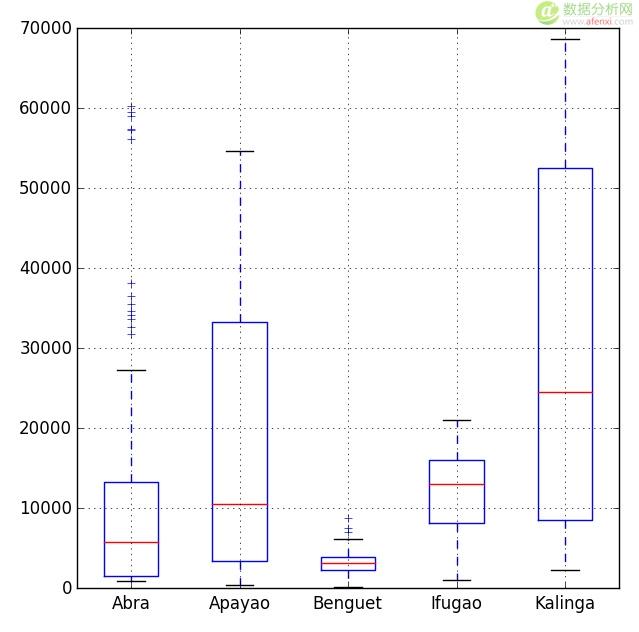
1 2 3 # Import the module for plotting import matplotlib.pyplot as plt plt.show(df.plot(kind = box))

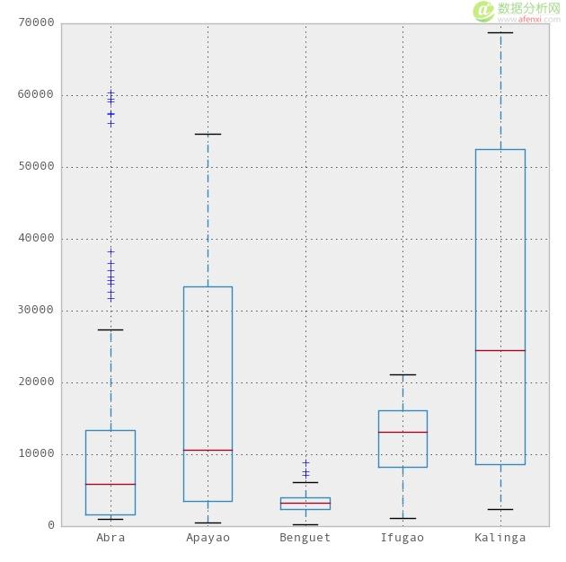
现在，我们可以用pandas模块中集成R的ggplot主题来美化图表。要使用ggplot，我们只需要在上述代码中多加一行

1 2 3 import matplotlib.pyplot as plt pd.options.display.mpl_style = default # Sets the plotting display theme to ggplot2 df.plot(kind = box)

这样我们就得到如下图表：

比matplotlib.pyplot主题简洁太多。但是在本博文中，我更愿意引入seaborn模块，该模块是一个统计数据可视化库。因此我们有：

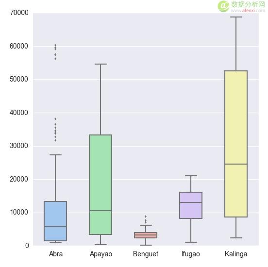
1 2 3 4 # Import the seaborn library import seaborn as sns # Do the boxplot plt.show(sns.boxplot(df, widths = 0.5, color = "pastel"))

多性感的盒式图，继续往下看。

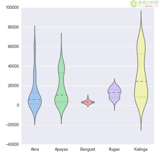
1 plt.show(sns.violinplot(df, widths = 0.5, color = "pastel"))

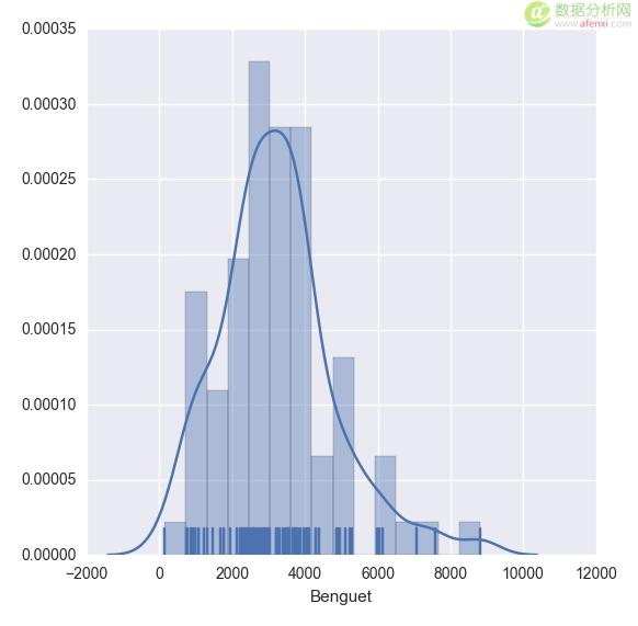
1 plt.show(sns.distplot(df.ix[:,2], rug = True, bins = 15))

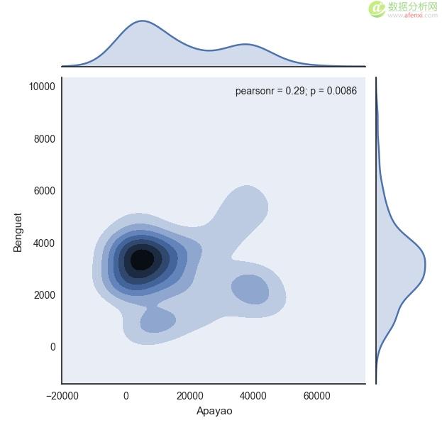
1 2 with sns.axes_style("white"):     plt.show(sns.jointplot(df.ix[:,1], df.ix[:,2], kind = "kde"))

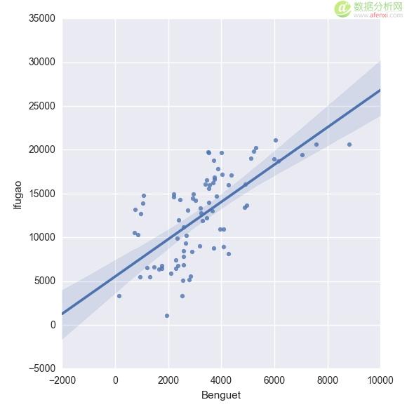
1 plt.show(sns.lmplot("Benguet", "Ifugao", df))

创建自定义函数

在Python中，我们使用def函数来实现一个自定义函数。例如，如果我们要定义一个两数相加的函数，如下即可：

1 2 3 4 5 6 7 def add_2int(x, y):     return x + y print add_2int(2, 2) # OUTPUT 4

顺便说一下，Python中的缩进是很重要的。通过缩进来定义函数作用域，就像在R语言中使用大括号

本文由 伯乐在线 - Den 翻译。英文出处：alstatr.blogspot.ca。

原创文章，作者：数据特工，如若转载，请注明出处：《如何通过Python来开始数据分析》http://www.afenxi.com/post/6789