一个自动化解决数据科学问题的python工具

摘要：机器学习中最乏味的部分就是调整超参数（简称调参）。

机器学习经常被吹捧为:

A field of study that gives computers the ability to learn without being explicitly programmed.

尽管这是一个常见的说法,在这个领域工作的人都知道设计有效的机器学习系统是一个乏味的过程,通常需要对机器学习算法有相当的经验,问题领域的专业知识，以及蛮力搜索来完成。因此,与机器学习爱好者试图让我们相信的相反,机器学习仍然需要大量的编程。

在本文中,我们要经历机器学习流程(pipline)设计中三个乏味的过程,但却如此重要。之后,我们将演示工具来遍历之前的过程,来体现智能自动化的机器学习流程设计,这样我们就可以花时间在数据科学的更有趣的方面。

模型超参数的优化是很重要的

机器学习中最乏味的部分就是调整超参数（简称调参）。

支持向量机要求我们选择理想的内核,内核的参数,和惩罚参数c .人工神经网络需要我们调整隐藏层的数量,隐藏节点的数量,以及更多的超参数。甚至随机森林也需要我们调整的树的数量以使得结果最好。

所有这些超参数可以对模型的效果产生重大影响。例如,我们使用MNIST手写的数字数据集来说明：

如果我们使用随机森林分类器（scikit-learn 默认的 10个树作为参数）：

In [5]:

import pandas as pd import numpy as np from sklearn.ensemble import RandomForestClassifier from sklearn.cross_validation import cross_val_score mnist_data = pd.read_csv(https://raw.githubusercontent.com/rhiever/Data-Analysis-and-Machine-Learning-Projects/master/tpot-demo/mnist.csv.gz, sep= , compression=gzip) cv_scores = cross_val_score(RandomForestClassifier(n_estimators=10, n_jobs=-1), X=mnist_data.drop(class, axis=1).values, y=mnist_data.loc[:, class].values, cv=10) print(cv_scores) print(np.mean(cv_scores))

[ 0.94118487 0.96159338 0.9486008 0.94043708 0.94971429 0.94056294 0.94698485 0.94197513 0.93982276 0.95683248] 0.946770856298

其交叉验证效果达到了94.7%，如果我们将参数调整到100棵树，效果会怎么样呢？

cv_scores = cross_val_score(RandomForestClassifier(n_estimators=100, n_jobs=-1),X=mnist_data.drop(class, axis=1).values, y=mnist_data.loc[:, class].values, cv=10) print(cv_scores) [ 0.96259814 0.97829812 0.9684466 0.96700471 0.966 0.96399486 0.97113461 0.96755752 0.96397942 0.97684391] print(np.mean(cv_scores)) 0.968585789367

这样一个小变化,我们将交叉验证精度的平均值从94.7%提高到了96.9%。如果我们的模型为美国邮政服务，那么这个小改善可以转化为成千上万的附加数字分类正确。

因此不要使用默认设置。超参数的调整对每个机器学习项目至关重要。

模型选择是重要的

我们都希望喜欢的模型很好地运用在每个机器学习问题中,但是不同的模型更适合不同的问题。

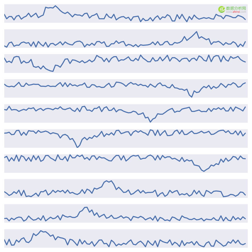
例如，我们在一个信号处理问题时,我们需要对时间序列中的“山”或“谷”进行分类:

我们应用“tuned”随机森林来解决问题:

import pandas as pd import numpy as np from sklearn.ensemble import RandomForestClassifier from sklearn.linear_model import LogisticRegression from sklearn.cross_validation import cross_val_score hill_valley_data = pd.read_csv(https://raw.githubusercontent.com/rhiever/Data-Analysis-and-Machine-Learning-Projects/master/tpot-demo/Hill_Valley_without_noise.csv.gz, sep= , compression=gzip) cv_scores = cross_val_score(RandomForestClassifier(n_estimators=100, n_jobs=-1), X=hill_valley_data.drop(class, axis=1).values, y=hill_valley_data.loc[:, class].values, cv=10) print(cv_scores) [ 0.64754098 0.64754098 0.57024793 0.61983471 0.62809917 0.61983471 0.70247934 0.59504132 0.49586777 0.65289256] print(np.mean(cv_scores)) 0.617937948787

然后我们会发现随机森林并不适合这样的信号处理任务，其交叉验证的精度平均水平才仅61.8%.

如果我们尝试不同的模型,例如逻辑回归,会怎么样呢?

cv_scores=cross_val_score(LogisticRegression(),X=hill_valley_data.drop(class, axis=1).values,y=hill_valley_data.loc[:, class].values,cv=10) print(cv_scores) [ 1. 1. 1. 0.99173554 1. 0.98347107 1. 0.99173554 1. 1. ] print(np.mean(cv_scores)) 0.996694214876

我们会发现逻辑回归非常适合这个信号处理任务,并且很容易达到近100%交叉验证精度同时又没有任何超参数调优。

因此对工作中的机器学习任务尝试各种不同的机器学习模型。尝试——调参-不同的机器学习模型尽管乏味但确是机器学习流程设计中至关重要的一步。

特征预处理是非常重要的

正如前面的两个例子中我们所看到的,机器学习模型的性能也受特征形式的影响。因此机器学习流程中的特征预处理，就是通过重塑特征的方式使数据集更容易被模型分类。

例如，我们用之前“山”或“谷”的一个更难一点的版本（加了噪声）来说明：

我们使用一个tuned的随机森林模型来解决这个问题：

import pandas as pd import numpy as np from sklearn.ensemble import RandomForestClassifier from sklearn.decomposition import PCA from sklearn.pipeline import make_pipeline from sklearn.cross_validation import cross_val_score hill_valley_noisy_data = pd.read_csv(https://raw.githubusercontent.com/rhiever/Data-Analysis-and-Machine-Learning-Projects/master/tpot-demo/Hill_Valley_with_noise.csv.gz, sep= , compression=gzip) cv_scores = cross_val_score(RandomForestClassifier(n_estimators=100, n_jobs=-1), X=hill_valley_noisy_data.drop(class, axis=1).values, y=hill_valley_noisy_data.loc[:, class].values, cv=10) print(cv_scores) [ 0.52459016 0.51639344 0.57377049 0.6147541 0.6557377 0.56557377 0.575 0.575 0.60833333 0.575 ] print(np.mean(cv_scores)) 0.578415300546

我们再次发现其交叉验证的平均值只有57.8%，令人失望。

然而，如果我们先通过主成分分析来降噪，

cv_scores = cross_val_score(make_pipeline(PCA(n_components=10),RandomForestClassifier(n_estimators=100,n_jobs=-1)),X=hill_valley_noisy_data.drop(class, axis=1).values,y=hill_valley_noisy_data.loc[:, class].values,cv=10) print(cv_scores) [ 0.96721311 0.98360656 0.8852459 0.96721311 0.95081967 0.93442623 0.91666667 0.89166667 0.94166667 0.95833333] print(np.mean(cv_scores)) 0.93968579235

我们会发现其结果惊人的提高到94%。

总结：为您的数据探索各种特征的表示方法。机器学习不同于人类,特征表示对我们可能有意义而对机器没有意义。

利用TPOT 自动化解决数据分析

总结一下我们目前学到的关于有效的机器学习系统设计,我们应该:

调整超参数 尝试不同的模型 探索特征不同的表示方式

同时我们也考虑下面几点：

每个模型都有非常多的超参数 机器学习的模型也很多 各种各样的数据特征预处理的方法也极其丰富

这就是为什么设计有效的机器学习系统如此乏味。这也是为什么我和我的合作者TPOT创建一个开源的Python工具,智能自动化的处理整个过程。

如果您的数据集与scikit-learn兼容,那么TPOT会自动优化的进行一系列特征预处理器和模型测试,最大化数据集上的交叉验证精度。例如,如果我们希望TPOT解决带扰动的“山”和“谷”的分类问题:

import pandas as pd from sklearn.cross_validation import train_test_split from tpot import TPOT hill_valley_noisy_data = pd.read_csv(https://raw.githubusercontent.com/rhiever/Data-Analysis-and-Machine-Learning-Projects/master/tpot-demo/Hill_Valley_with_noise.csv.gz, sep= , compression=gzip) X = hill_valley_noisy_data.drop(class, axis=1).values y = hill_valley_noisy_data.loc[:, class].values X_train, X_test, y_train, y_test = train_test_split(X, y, train_size=0.75, test_size=0.25) my_tpot = TPOT(generations=10) my_tpot.fit(X_train, y_train) print(my_tpot.score(X_test, y_test)) 0.960352039038

根据你使用的电脑，一般10 generations的 TPOT大概要5分钟。这期间你可以做任何你想做的事情，放松一下。

经过5分钟的优化,TPOT会发现一种达到96%的交叉验证准确性，比我们之前手动创建的流程更好!

如果我们想知道它具体是什么，TPOT可以自动化的导出具体的 scikit-learn 代码：使用 export() 命令

my_tpot.export(exported_pipeline.py)

其具体结果如下：

import pandas as pd from sklearn.cross_validation import train_test_split from sklearn.linear_model import LogisticRegression # NOTE: Make sure that the class is labeled class in the data file tpot_data = pd.read_csv(https://raw.githubusercontent.com/rhiever/Data-Analysis-and-Machine-Learning-Projects/master/tpot-demo/Hill_Valley_with_noise.csv.gz, sep= , compression=gzip) training_indices, testing_indices = train_test_split( tpot_data.index,stratify=tpot_data[class].values,train_size=0.75,test_size=0.25) result1 = tpot_data.copy() # Perform classification with a logistic regression classifier lrc1 = LogisticRegression(C=0.0001) lrc1.fit(result1.loc[training_indices].drop(class, axis=1).values, result1.loc[training_indices, class].values) result1[lrc1-classification] = lrc1.predict(result1.drop(class, axis=1).values)

它告诉我们一个 tuned logistic 回归也许是这个问题的最优模型。

我们设计TPOT是一个衔接完整的机器学习系统，可以作为一个替代任何您目前正在使用的scikit-learn的工作流模型。

如果TPOT听起来像你所苦苦寻找的工具，下面几个连接也许对你十分有用：

TPOT repository on GitHub [TPOT documentation] (http://rhiever.github.io/tpot/) TPOT installation instructions TPOT example code

和往常一样,有问题请随时联系我。

原文地址： http://www.randalolson.com/2016/05/08/tpot-a-python-tool-for-automating-data-science/

作者：Randy Olson

翻译： lan